| Include Page | ||||
|---|---|---|---|---|
|
| Hide_comments |
|---|
Table of contents
| Table of Contents | ||
|---|---|---|
|
Terminology
- ABR - a router located at OSPF areas bordersthe border of an OSPF area.
- ASBR - a router located at the autonomous system border and connected to the an external networksnetwork.
- DR - designated router.
- BDR - backup designated router.
- LSA - link state advertisement.
- LSDB - link state data basedatabase.
- DBD - Short description of the LSDB short description.
- LSR - link state advertisement request.
- LSU - link state update, reply on LSR.
- LSAck - acknowledgment upon receiving an LSU.
The OSPF protocol
OSPF (Open Shortest Path First) - a dynamic routing protocol based on an algorithm that constructs a shortest path tree. The OSPF protocol has the following features:
- OSPF was developed by the IETF community in 1988. Since it is an open protocol, it can be used in heterogeneous networks built using equipment from different manufacturers.
- Today, two versions of the OSPF protocol are relevant: version 2 for IPv4 networks, described in RFC 2328, and version 3 for IPv6 networks, described in RFC 2740. InfiNet The InfiNet devices support the operation of the IPv4 protocol, therefore, in this article only OSPF version 2 will be described.
- OSPF is a link state dynamic routing protocol.
- OSPF is an internal routing protocol, i.e. used to exchange routing information within an autonomous system (AS).
- The OSPF service messages are encapsulated in IP packets. The upper layer protocol field is set to 89.
Two multicast addresses are reserved for OSPF: 224.0.0.5 and 224.0.0.6. These addresses are described below (see setting up neighborhood relations and DR and BDR selection algorithm). - The distance value for the OSPF protocol is 110.
...
The number of autonomous system routers that use OSPF to exchange routing information can be large. This leads to a high load of the communication channels because of the large number of OSPF service messages. To reduce the amount of the transmitted service information, the OSPF protocol divides the autonomous system into areas.
...
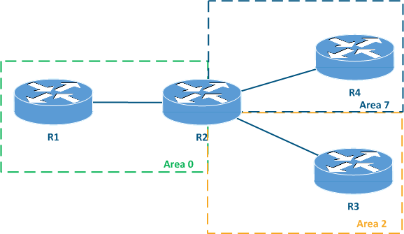
It is not necessary to use sequential identifiers for the areas. For example, the network can include areas with the identifiers 0, 2 and 7 (Figure 1a).
...
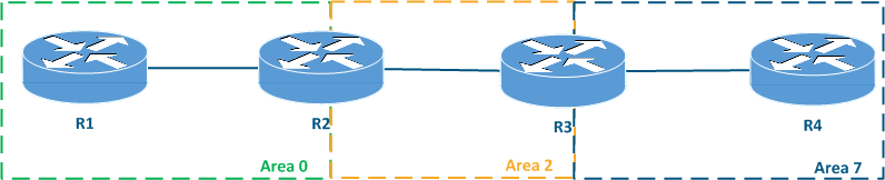
The area with the identifier 0.0.0.0 has a special role - this area is called the backbone area. The backbone area is a requirement for the OSPF operation. Each area must be directly connected to the backbone area, i.e. a scheme in which some area is connected to another one without having a direct connection to the backbone is prohibited (Figure 1b).
| Center |
|---|
Figure 1a - Permitted Allowed network scheme with multiple OSPF areas
Figure 1b - Prohibited network scheme with multiple OSPF areas |
...
Router types
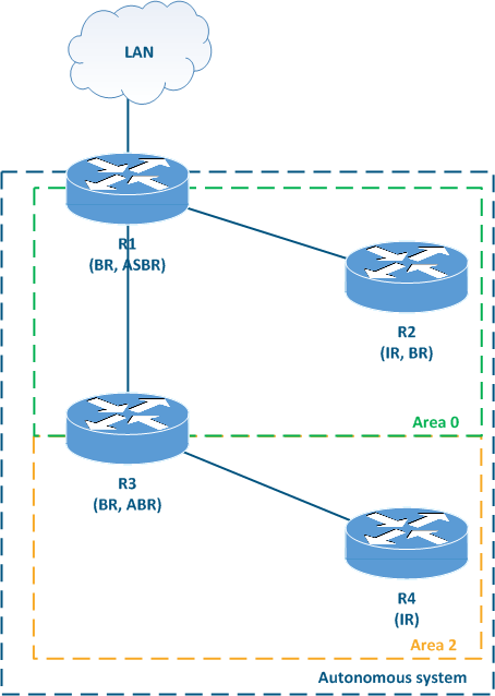
Depending on the router's place in the network, the following types of devices are distinguished (Figure 2):
- Internal router (IR): a router which has all its interfaces associated with the same area. Routers R2 and R4 are internal.
- Backbone router (BR): a router with an interface connected to the backbone area. Routers R1, R2 and R3 are backbone routers.
- Area border router (ABR): a router having interfaces associated with different OSPF areas. Router R3 is ABR because it is located at the border of areas 0 and 2.
- ,Autonomous system border router (ASBR): a router connected to an external network. Router R1 is ASBR because it is connected to a third party LAN.
| Center |
|---|
Figure 2 - Network scheme with different router types |
OSPF's operation
The OSPF 's operation process follows the below steps. Some steps will require a detailed explanation which is provided in the sections below.
- Step 1: OSPF protocol launching. The configuration of the devices includes a list of interfaces that will participate in the OSPF's protocol operation, associated with the area identifiers to which these interfaces are connected. Upon this configuration, OSPF is launched.
- Step 2: Setting up neighboring relations. The device makes an attempt to find other routers and establish neighboring relations using the list of interfaces defined in step 1.
- Step 3: Role distribution. To reduce the service traffic volume in the broadcast network segments, a designated router (DR) is elected, which will be the central point for routing information exchange inside the broadcast segment.
- Step 4: Link state database (LSDB) synchronization. OSPF requires that each router has the same set of routing information, which implies the synchronization of the link state databases.
- Step 5: Building the shortest paths tree (SPT). Dijkstra's algorithm is applied to the routing information obtained in step 4 in order to build the shortest path tree. The root of the tree is the device on which the algorithm is running and the branches are the known destination networks, obtained from the other routers. Thus, each device has a set of paths to each network, optimized using the metric.
- Step 6: Export of the routes to the FIB. The set of routes obtained in step 5 is stored in the RIB, so that the device can perform additional optimizations by comparing the Distance values for the routing information obtained from different sources. The best routes obtained during the comparison are placed in the FIB and used to transfer the user and the service data.
- Step 7: Continuous monitoring of the network's state. Dynamic routing protocols perform a constant link state monitoring, because the routing table of all the devices must be kept up to date.
| Anchor | ||||
|---|---|---|---|---|
|
Two processes actions are performed when the OSPF service is launchinglaunched: the selection of a the router identifier and the definition of a list of interfaces that will participate in OSPF.
The router has a 32-bit identifier, which is usually written in the IP address format. Usually, the identifier is not connected related with the device's IP address and can be set manually. If the identifier is not set manually, it will be automatically selected as the highest IP address of the device. In case of manual setting of the ID selection, it is recommended to set it in the IP address of the loopback0 interface. This will help to identify the devices easier and to speed up the diagnostic of the network problems.
During the automatic router ID selection, the Infinet InfiNet device generates a special address from the 224. *. *. * multicast subnet, associated with the router's serial number. This helps to avoid the redefinition necessity of redefining the router ID when the IP address or the network interface are removed.
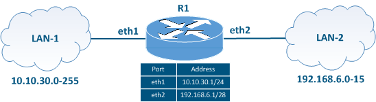
The set of interfaces that will take part into the OSPF 's protocol operation is determined according to based on the following rules:
- the range of IP addresses (or subnet) and their association with a specific area are specified in the configuration of the device (router);
- the network interfaces having IP addresses included in the specified range will take part into the OSPF process and become associated with the specified area. Note: not only the IP address of the interface is checked to see if it included in the specified range, but the whole network associated with the interface (see the example below).
...
| Center | ||||||||||||||||
|---|---|---|---|---|---|---|---|---|---|---|---|---|---|---|---|---|
Figure 3 - Router with two network interfaces |
...
The list of networks that are assigned to the interfaces is defined when OSPF starts. in addition, OSPF can advertise routes to towards other networks, that were added to the device's routing table. The announcement of such routes is called redistribution. These routes are external to OSPF.
The routing sources for redistribution can be other dynamic routing protocols, static entries or directly attached connected networks not added to OSPF.
...
The routing information exchange is possible only after the establishment of the neighboring relations between the routers. Two routers having a common link will establish a neighborhood relationship neighboring relation if the following parameters match:
- the network address of the interface towards a potential neighbor;
- MTU value on the interfaces towards a potential neighbor;
- area ID and area type;
- authentication parameters;
- Hello messages interval and Router dead interval (see step 1 of setting up neighboring relations).
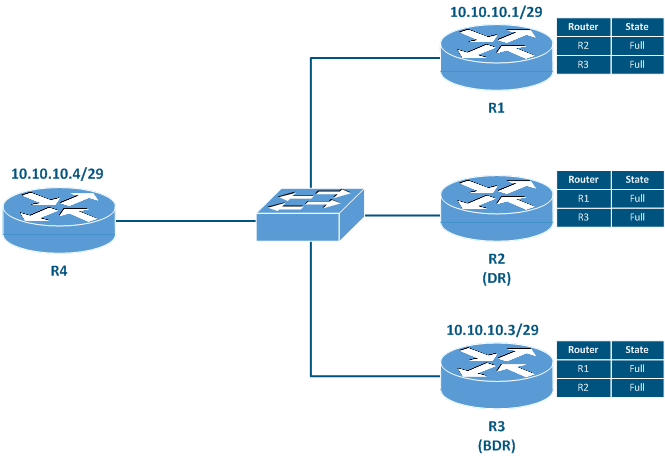
Neighboring The neighboring relations are established in several steps. Let's look at an example (Figure 4a): the network consists of three routers R1, R2 and R3 connected to the switch. Neighboring relations are established between the routers ( the R2 router is selected as the designated router (DR), R3 as the backup designated router (BDR) ). Router R4 will be added to the network scheme and let's assume that the conditions for establishing neighboring relations are met.
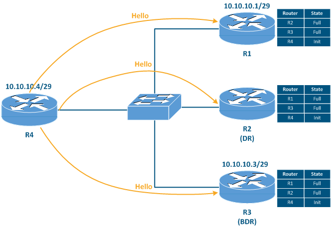
Step 1: The R4 router sends Hello messages to the multicast address 224.0.0.5 (Figure 4b). This address is supported by all the devices running OSPF. Hello messages are sent from all the interfaces defined during the OSPF launching with a specified periodicity. The default Hello message broadcast interval is 10 seconds. Hello messages are an indicator of the connection with the neighbor, therefore, if no Hello messages are received from the neighbor during the Router dead interval, the device is marked as unavailable. By default, the Router dead interval is equal to four Hello message intervals.Anchor hello_neighboor hello_neighboor - Step 2: The R1, R2 and R3 routers receive the Hello message from R4 and add it to the list of neighbors with the Init status (Figure 4b).
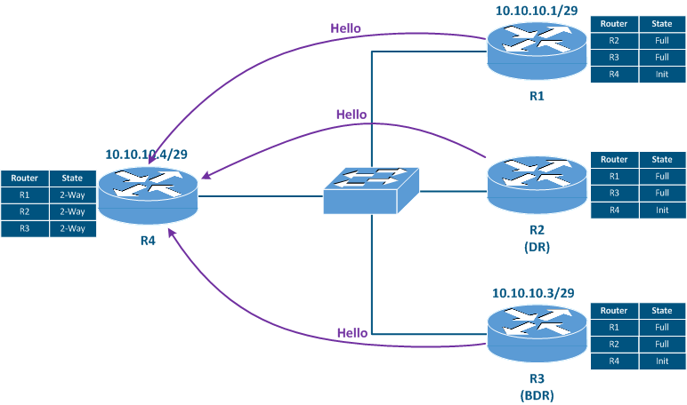
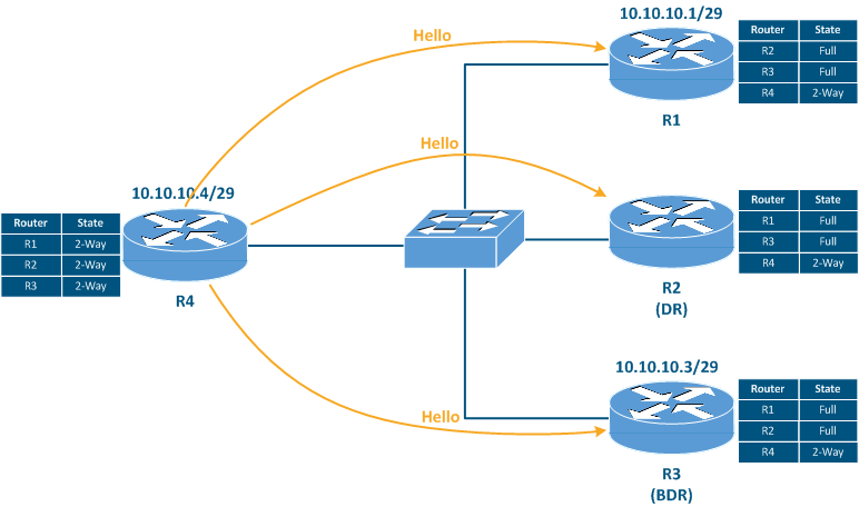
- Step 3: According to the internal timers, the R1, R2, R3 routers send Hello messages to router R4 (Figure 4c). Since the Hello messages contain a list of neighbors, the messages sent to R4 contain its ID. This means that router R4 can add all routers therouters to the list of neighbors with the 2-Way status, skipping the Init status. Then R4 will generate Hello messages for the routers, where it will indicate routers R1, R2 and R3 as neighbors, which will allow R1, R2 and R3 to change the status for R4 from Init to 2-Way (Figure 4d).
- Step 4: in broadcast segments (Ethernet, MINT, etc.), routers designated as a primary router (DR) and a backup router (BDR) must be selectedelected. The rest of the routers will be set as with the DROther role. This mechanism is intended to reduce the amount of the overhead traffic amount: each DROther will exchange routing information only with the DR and the BDR. The DR and the BDR selection election algorithm is describer below. Note that the roles are not assigned to a device, but to an interface, so a router that has multiple interfaces in different broadcast segments may be DR in one segment and DROther in the other.
- Step 4a: let R2 be DR and R3 - BDR as it was before R4 has been added to the network. The routers R1 and R4 have the DROther role, so the status between them will remain 2-Way.
- Step 5: The pairs of routers R2-R4 and R3-R4 distribute the roles of master and slave among themselves, the status of their relationship relation becoming ExStart.
- Step 6: The Master device first begins the exchange of service messages with a brief DBD route database description. During the exchange of such messages, the relationshiprelation's status is set to Exchange.
- Step 7: The devices receive the short route database description from the neighbor and generate requests for detailed information about the unknown networks. These messages are called LSRs.
- Step 7a: An LSU is the answer to the LSR. LSUs contain detailed information about the requested routes.
- Step 7b: The device receiving an LSU will generate an acknowledgment of the received information. This message is called LSAck.
- Step 7c: The routing information base containing all the gathered routing information is called LSDB and the exchange of LSDB service messages changes the relationshiprelation's status to Loading.
- Step 8: After the LSDB is synchronized on all the devices, the relationship between routers R4-R2 and R4-R3 is set to the Full status (Figure 4e). Note that the DR and BDR establish Full relationships relations with all the routers in the segment.
| Center |
|---|
Figure 4a - The R4 router was added to the network scheme
Figure 4b - R4 sends Hello messages
Figure 4c - R1, R2, R3 send Hello messages
Figure 4d - 2-Way relationships relations were established
Figure 4e - Full relations were established by R4 with the DR and the BDR |

...
In each broadcast segment where OSPF is running, DR and BDR elections are performed. The elections are carried out according to the following rulescriteria:
- Interface priority value: the DR is the router with the highest priority value, the BDR is the router following the DR in priority value, the DROther's DROthers are the remaining routers. The priority parameter is configured on the interface that is connected to the broadcast segment. The priority is set manually by the network administrator and it can be in the range from 0 to 255. By default, the priority is 1. If the router interface priority value is set to 0, then that router does not participate in the DR and BDR elections.
- Router-id value: The DR is the router with the highest Router-id value, the BDR is the router following the DR in Routerin the Router-id value, the DROther's DROthers are the remaining routers. The Router-id is unique, so the router ID comparison is used when the priorities are equal, which ensures the distribution of the roles.
The group address 224.0.0.6 is associated with the DR and the BDR devices, which is used for LSDB synchronization. The devices having DR and BDR roles establish a Full relationship relation with each router in the broadcast segment and require higher device performance demands compared to the DROthers. Since the device's hardware performance can become a bottleneck, it should be taken into account during network planning. Interface prioritization should be set in order to ensure a predictable selection of the highest performing devices as DR and BDR.
The main function of the DR is the routing information exchange in the broadcast segment. The main function of the BDR is to monitor the DR's state and, if it fails, to change the role to DR. Since each DROther establishes a Full relationship relation with both the DR and the BDR, the LSDB on the BDR is synchronous with the DR, so the BDR can start performing the DR's functions without timing database synchronization timing delays. If the BDR becomes DR, then the BDR is selected among the DROthers according to the algorithm described above.
...
| Center | ||||||||||||||||||||||||||||||||
|---|---|---|---|---|---|---|---|---|---|---|---|---|---|---|---|---|---|---|---|---|---|---|---|---|---|---|---|---|---|---|---|---|
|
| Center |
|---|
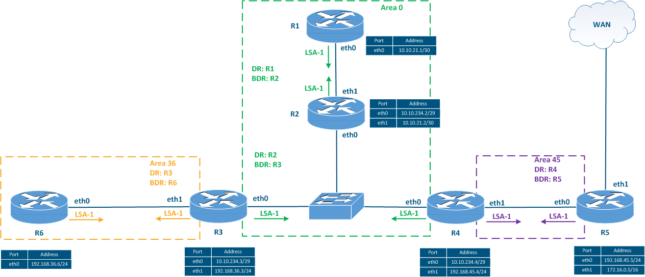
Figure 5a - Network scheme used for analyzing the LSA types analyzing
Figure 5b - Distribution of the LSA type 1 distribution
Figure 5c - Distribution of the LSA type 2 distribution
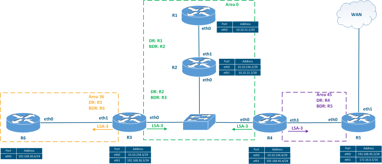
Figure 5d - Distribution of the LSA type 3 distribution
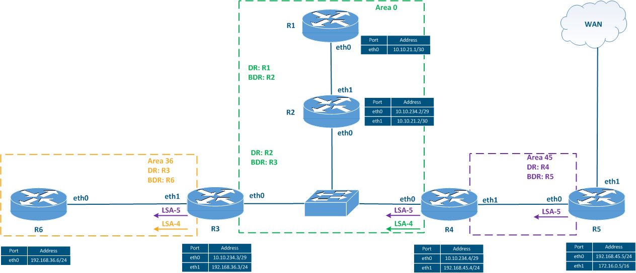
Figure 5e - Distribution of the LSA type 4 and of the LSA type 5distribution |


Building the shortest
...
path tree
After the LSDB synchronization, each router performs a shortest paths path tree calculation using Dijkstra's algorithm.
In the networks with channel having redundancy implemented, the LSDB contains announcements about 1about the same network received from different sources. Such routes are transmitted to the RIB in the following order:
- Intra-area routes: routes distributed within the same area using LSA types 1 and 2.
- Inter-area routes: routes received from neighboring areas using LSA type 3.
- External Type 1 external routes type 1: routes to external networks received from the ASBR. The routes route metric for this type of routes is counted as the metrics sum of the metric set by the ASBR during the announcement plus the metric of a the path to the ASBR.
- External Type 2 external routes type 2: are similar to External routes the type 1 external routes, with a different method of for the metric calculation. The metric is equal to the value set by the ASBR during the announcement and does not include the path to the ASBR.
- Route metric Metric value: for two routes to the same network received from sources of the same type, the metric values are compared. The route with the lower metric value will be added to the RIB.
| Anchor | ||||
|---|---|---|---|---|
|
...
Area types
The way to reduce the OSPF service traffic volume is to use different types of areas. The OSPF protocol provides for the following types of areas:
- Normal;
- Stub;
- Totally Stub;
- NSSA;
- Totally NSSA.
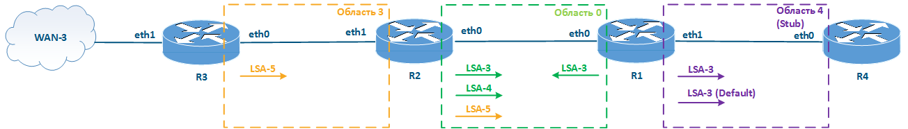
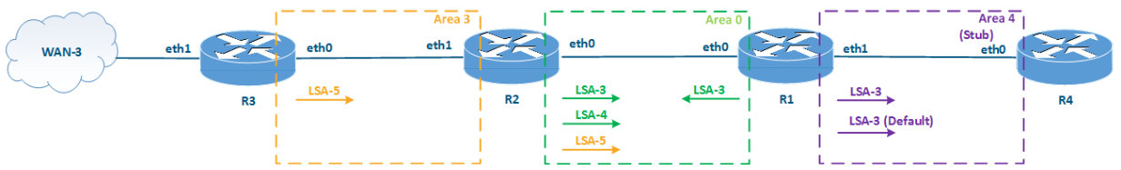
Let's look at the main features of different areas area types at using the example via the following scheme in (Figure 6): routers R1, R2, R3 and R4 are connected in sequence chain with each other, forming three OSPF areas. Routers R3 and R4 have external links. In each example, we will change the type of area 4 and analyze the LSA types associated with that area. In these examples, the details of LSA's not connected related with area 4 and LSA of types the type 1 and 2 LSAs will be omitted because they are distributed within areas of any area type.
| Center |
|---|
Figure 6 - Network scheme used for the description of the area types description |

Normal
Normal areas do not change the LSA propagation of the LSAs and the processing logic described above (Figure 7a). This area type is used by default. The backbone area is a special case of the Normal area.
...
- The Stub area cannot have external links. Thus LSA types 5 and 4 are prohibited in the Stub area.
- Stub The stub area's routing information is distributed to the neighboring areas using LSA type 3.
- LSA Type 3 messages about the networks in third different areas are distributed in the Stub area, similarly to the Normal areas.
- When an LSA type 5 from third areas, when it a different area enters the Stub area, it is converted to LSA type 3 with the default route information.
Stub areas are used in LAN segments that have no connection to with the external linksnetworks, but the routers in this area must receive full routing information from the neighboring areas in full. The Using Stub areas using allows to obtain a small increase in performance increasment by reducing the LSA number and to protect the network from attacks that involve connecting the router to from the external network segment.
| Center |
|---|
Figure 7b - LSA distribution in the Stub area |
...
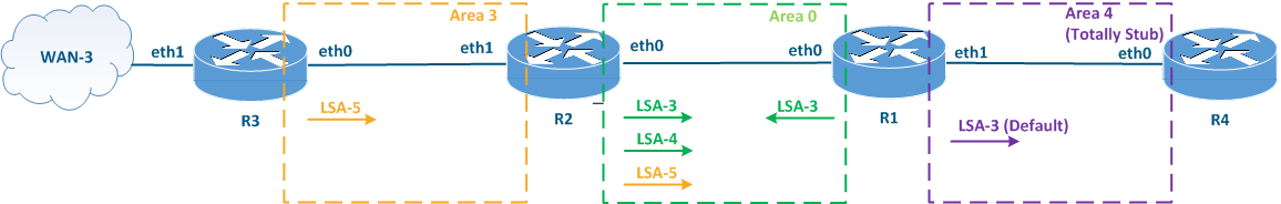
The Totally Stub area behaves similarly to the Stub area with one exception: LSA's of types 3 and 5 from the neighboring areas are replaced with one LSA type 3 with a default route (Figure 7c).
Totally Stub areas area applications are similar to the ones of the Stub area, but the routers in a totally stub area routers will not have all the routing information about the neighboring areas. This will give offers a significant performance increase, as Totally Stub area routers will use a single default route to transmit data to the neighboring areas.
| Center |
|---|
Figure 7c - LSA distribution in the Totally Stub area |
| Anchor | ||||
|---|---|---|---|---|
|
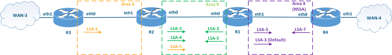
The NSSA area has the characteristics of similar to the Stub area with one exception: the NSSA can have an external link (Figure 7d). Since LSA type 5 which are is used to distribute routing information about the external links, are is prohibited in Stub areas, NSSA areas use LSA type 7 for this purpose. This LSA type has the same structure as LSA type 5, but it is permitted for distribution in NSSA areas. At the area border, the ABR converts the LSA type 7 to LSA type 5, setting itself as the routing source. Since the ABR performing the LSA conversion become becomes the source, there is no need to create generate an additional type 4 LSA.
Usually, the NSSA area using usage is a result of the network's development: connecting an external communication channel to the Stub area requires changing its type to NSSA.
| Center |
|---|
Figure 7d - LSA distribution in the NSSA area |
Totally NSSA
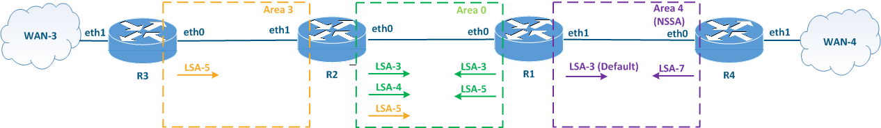
Totally NSSA areas behave similarly to the NSSA areas with the one exception: only one type 3 LSA with a default route is exported to the Totally NSSA area (Figure 7e).
Totally NSSA areas is are a result of the network development: connecting an external link to a Totally Stub area requires changing the type of the area type to Totally NSSA.
| Center |
|---|
Figure 7e - LSA distribution in the Totally NSSA area |
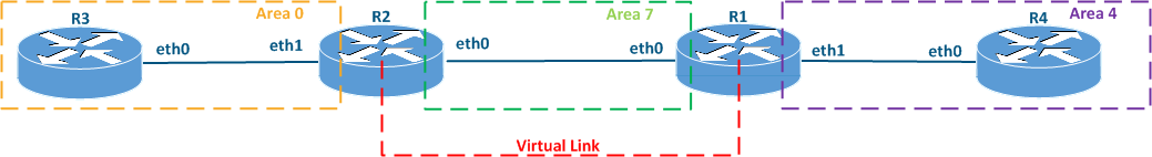
Virtual link
One of the OSPF principles is possibility to always connect two non-backbone areas only through the backbone area. Despite that, as a result of the historical development, the structure of some networks does not match to with this principle. Bringing such networks up to the OSPF requirements backbone can be costly, so OSPF has been extended with the virtual link concept.
...
- A virtual link is a logical connection configured on two ABRs, one of which is connected to the backbone area. Routers R1 and R2 are ABRs on which a virtual network interface is created , and R2 is connected to the backbone area via eth1interfacethe eth1 interface.
- The virtual link is the interface used by R2 to connect area 4. All LSA types are distributed over the virtual link , like through a normal interface.
- The area that is common for two ABRs organizing sharing a virtual link is called a transit area. In the example below, area 7 is the transit area.
- Transit The transit area should have Normal have the Normal type. It is not possible to establish a virtual link through Stub or NSSA areas.
| Center |
|---|
Figure 8 - Network scheme with a virtual link |
OSPF's protocol features
The OSPF protocol features can be represented in following waysummarized as follows:
- Open implementation: OSPF is an open protocol, so it can be used on by equipment from different manufacturers.
- Easy configuration: in small networks, the protocol can be started with only two commands.
- Flexible configuration: wide the wide protocol tools tool set allows to implement many network schemes.
- Scalability, fault tolerance, balancing, efficiency: similar to the ODR, OSPF has the advantages of a dynamic routing protocolsprotocol.
- High entry threshold: understanding the OSPF terminology and logic is time consuming.
| Tip | ||
|---|---|---|
| ||
The examples of on how to configure OSPF configuration are on present in the document child page: OSPF protocol's configuration. |
Additional materials
Webinars
...